Popcorn Hacks
Popcorn Hack 1: Find Students with Scores in a Range
pip install pandas
Collecting pandas
Using cached pandas-2.2.3-cp313-cp313-macosx_10_13_x86_64.whl.metadata (89 kB)
Requirement already satisfied: numpy>=1.26.0 in /Users/maryamabdul-aziz/vscode/maryam_2025/venv/lib/python3.13/site-packages (from pandas) (2.2.4)
Requirement already satisfied: python-dateutil>=2.8.2 in /Users/maryamabdul-aziz/vscode/maryam_2025/venv/lib/python3.13/site-packages (from pandas) (2.9.0.post0)
Requirement already satisfied: pytz>=2020.1 in /Users/maryamabdul-aziz/vscode/maryam_2025/venv/lib/python3.13/site-packages (from pandas) (2025.1)
Requirement already satisfied: tzdata>=2022.7 in /Users/maryamabdul-aziz/vscode/maryam_2025/venv/lib/python3.13/site-packages (from pandas) (2025.1)
Requirement already satisfied: six>=1.5 in /Users/maryamabdul-aziz/vscode/maryam_2025/venv/lib/python3.13/site-packages (from python-dateutil>=2.8.2->pandas) (1.17.0)
Using cached pandas-2.2.3-cp313-cp313-macosx_10_13_x86_64.whl (12.5 MB)
Installing collected packages: pandas
Successfully installed pandas-2.2.3
[1m[[0m[34;49mnotice[0m[1;39;49m][0m[39;49m A new release of pip is available: [0m[31;49m25.0[0m[39;49m -> [0m[32;49m25.0.1[0m
[1m[[0m[34;49mnotice[0m[1;39;49m][0m[39;49m To update, run: [0m[32;49mpip install --upgrade pip[0m
Note: you may need to restart the kernel to use updated packages.
import pandas as pd

student_data = pd.DataFrame({
    'Name': ['Aditi', 'Brady', 'Charlotte', 'Daniel', 'Emily'],
    'Score': [92, 84, 78, 95, 82],
    'Grade': ['A', 'B', 'C', 'A', 'B']
})

# Complete the function to find all students with scores between min_score and max_score
def find_students_in_range(df, min_score, max_score):
    return df[(df['Score'] >= min_score) & (df['Score'] <= max_score)]

print(find_students_in_range(student_data, 80, 90))
    Name  Score Grade
1  Brady     84     B
4  Emily     82     B
PopCorn Hack 2: Calculate Letter Grades
import pandas as pd

student_data = pd.DataFrame({
    'Name': ['Aditi', 'Brady', 'Charlotte', 'Daniel', 'Emily'],
    'Score': [92, 84, 78, 95, 82],
    'Grade': ['A', 'B', 'C', 'A', 'B']
})

# Complete the function to add a 'Letter' column based on numerical scores
def add_letter_grades(df):
    def get_letter(score):
        if score >= 90:
            return 'A'
        elif score >= 80:
            return 'B'
        elif score >= 70:
            return 'C'
        elif score >= 60:
            return 'D'
        else:
            return 'F'

    df['Letter'] = df['Score'].apply(get_letter)
    return df

add_letter_grades(student_data)
| Name | Score | Grade | Letter | |
|---|---|---|---|---|
| 0 | Aditi | 92 | A | A |
| 1 | Brady | 84 | B | B |
| 2 | Charlotte | 78 | C | C |
| 3 | Daniel | 95 | A | A |
| 4 | Emily | 82 | B | B |
PopCorn Hack 3: Find the Mode in a Series
# Complete the function to find the most common value in a series
def find_mode(series):
    mode = series.mode()
    return mode

find_mode(pd.Series([1, 2, 2, 3, 4, 2, 5]))
0    2
dtype: int64
Homework Hacks
For this homework, you’ll work with a dataset of student performance and implement various list algorithms using both Python lists and Pandas.
Dataset: Pima Indians Diabetes Info
Algorithms
import pandas as pd
datas = pd.read_csv('/Users/maryamabdul-aziz/vscode/maryam_2025/_notebooks/data/diabetes.csv')

# Highest and lowest BMI
def get_extreme_bmi(datas):
    highest_bmi = datas[datas['BMI'] == datas['BMI'].max()]
    lowest_bmi = datas[datas['BMI'] == datas['BMI'].min()]
    return highest_bmi, lowest_bmi

# Difference between max and min for Glucose, BloodPressure, and BMI
def add_max_min_diff(datas):
    datas['MaxMinDiff'] = datas[['Glucose', 'BloodPressure', 'BMI']].max(axis=1) - \
                          datas[['Glucose', 'BloodPressure', 'BMI']].min(axis=1)
    return datas

# Patients with Glucose above the average
def get_above_avg_glucose(datas):
    avg_glucose = datas['Glucose'].mean()
    return datas[datas['Glucose'] > avg_glucose]

# Group by AgeGroup and Outcome, then calculate mean BMI and Glucose
def group_by_age_outcome(datas):
    datas = datas.copy()
    datas['AgeGroup'] = pd.cut(datas['Age'], bins=[20, 30, 40, 50, 60, 100],
                                labels=['20s', '30s', '40s', '50s', '60+'], right=False)
    grouped = datas.groupby(['AgeGroup', 'Outcome'])[['BMI', 'Glucose']].mean().reset_index()
    return grouped

# Correlation between Age and BMI
def age_bmi_correlation(datas):
    return datas['Age'].corr(datas['BMI'])

# Age group with highest average glucose
def age_group_with_highest_glucose(datas):
    datas = datas.copy()
    datas['AgeGroup'] = pd.cut(datas['Age'], bins=[20, 30, 40, 50, 60, 100],
                                labels=['20s', '30s', '40s', '50s', '60+'], right=False)
    glucose_by_age = datas.groupby('AgeGroup')['Glucose'].mean()
    return glucose_by_age.idxmax(), glucose_by_age

# Percentage of individuals with BMI > 30 (obese)
def percent_obese(datas):
    obese_count = datas[datas['BMI'] > 30].shape[0]
    total_count = datas.shape[0]
    return (obese_count / total_count) * 100

highest, lowest = get_extreme_bmi(datas)
datas = add_max_min_diff(datas)
glucose_above_avg = get_above_avg_glucose(datas)
grouped_stats = group_by_age_outcome(datas)
correlation = age_bmi_correlation(datas)
top_age_group, glucose_age_distribution = age_group_with_highest_glucose(datas)
obese_pct = percent_obese(datas)

print(highest, lowest)
print(datas)
print(glucose_above_avg)
print(grouped_stats)
print(correlation)
print(top_age_group, glucose_age_distribution)
print(obese_pct)
     Pregnancies  Glucose  BloodPressure  SkinThickness  Insulin   BMI  \
177            0      129            110             46      130  67.1

     DiabetesPedigreeFunction  Age  Outcome
177                     0.319   26        1        Pregnancies  Glucose  BloodPressure  SkinThickness  Insulin  BMI  \
9              8      125             96              0        0  0.0
49             7      105              0              0        0  0.0
60             2       84              0              0        0  0.0
81             2       74              0              0        0  0.0
145            0      102             75             23        0  0.0
371            0      118             64             23       89  0.0
426            0       94              0              0        0  0.0
494            3       80              0              0        0  0.0
522            6      114              0              0        0  0.0
684            5      136             82              0        0  0.0
706           10      115              0              0        0  0.0

     DiabetesPedigreeFunction  Age  Outcome
9                       0.232   54        1
49                      0.305   24        0
60                      0.304   21        0
81                      0.102   22        0
145                     0.572   21        0
371                     1.731   21        0
426                     0.256   25        0
494                     0.174   22        0
522                     0.189   26        0
684                     0.640   69        0
706                     0.261   30        1
     Pregnancies  Glucose  BloodPressure  SkinThickness  Insulin   BMI  \
0              6      148             72             35        0  33.6
1              1       85             66             29        0  26.6
2              8      183             64              0        0  23.3
3              1       89             66             23       94  28.1
4              0      137             40             35      168  43.1
..           ...      ...            ...            ...      ...   ...
763           10      101             76             48      180  32.9
764            2      122             70             27        0  36.8
765            5      121             72             23      112  26.2
766            1      126             60              0        0  30.1
767            1       93             70             31        0  30.4

     DiabetesPedigreeFunction  Age  Outcome  MaxMinDiff
0                       0.627   50        1       114.4
1                       0.351   31        0        58.4
2                       0.672   32        1       159.7
3                       0.167   21        0        60.9
4                       2.288   33        1        97.0
..                        ...  ...      ...         ...
763                     0.171   63        0        68.1
764                     0.340   27        0        85.2
765                     0.245   30        0        94.8
766                     0.349   47        1        95.9
767                     0.315   23        0        62.6

[768 rows x 10 columns]
     Pregnancies  Glucose  BloodPressure  SkinThickness  Insulin   BMI  \
0              6      148             72             35        0  33.6
2              8      183             64              0        0  23.3
4              0      137             40             35      168  43.1
8              2      197             70             45      543  30.5
9              8      125             96              0        0   0.0
..           ...      ...            ...            ...      ...   ...
759            6      190             92              0        0  35.5
761            9      170             74             31        0  44.0
764            2      122             70             27        0  36.8
765            5      121             72             23      112  26.2
766            1      126             60              0        0  30.1

     DiabetesPedigreeFunction  Age  Outcome  MaxMinDiff
0                       0.627   50        1       114.4
2                       0.672   32        1       159.7
4                       2.288   33        1        97.0
8                       0.158   53        1       166.5
9                       0.232   54        1       125.0
..                        ...  ...      ...         ...
759                     0.278   66        1       154.5
761                     0.403   43        1       126.0
764                     0.340   27        0        85.2
765                     0.245   30        0        94.8
766                     0.349   47        1        95.9

[349 rows x 10 columns]
  AgeGroup  Outcome        BMI     Glucose
0      20s        0  29.852885  106.503205
1      20s        1  37.101190  140.642857
2      30s        0  30.923596  113.348315
3      30s        1  34.285526  139.315789
4      40s        0  33.318868  109.509434
5      40s        1  35.676923  136.984615
6      50s        0  30.221739  123.782609
7      50s        1  32.094118  151.441176
8      60+        0  27.165217  131.391304
9      60+        1  31.755556  155.777778
0.03624187009229404
50s AgeGroup
20s    113.744949
30s    125.309091
40s    124.644068
50s    140.280702
60+    138.250000
Name: Glucose, dtype: float64
60.546875


/var/folders/93/y55vzx413xxdrd4m_6cv_rmm0000gn/T/ipykernel_13033/3696993698.py:26: FutureWarning: The default of observed=False is deprecated and will be changed to True in a future version of pandas. Pass observed=False to retain current behavior or observed=True to adopt the future default and silence this warning.
  grouped = datas.groupby(['AgeGroup', 'Outcome'])[['BMI', 'Glucose']].mean().reset_index()
/var/folders/93/y55vzx413xxdrd4m_6cv_rmm0000gn/T/ipykernel_13033/3696993698.py:38: FutureWarning: The default of observed=False is deprecated and will be changed to True in a future version of pandas. Pass observed=False to retain current behavior or observed=True to adopt the future default and silence this warning.
  glucose_by_age = datas.groupby('AgeGroup')['Glucose'].mean()
Analytical Questions
import pandas as pd
datas = pd.read_csv('/Users/maryamabdul-aziz/vscode/maryam_2025/_notebooks/data/diabetes.csv')
def master_function(datas):
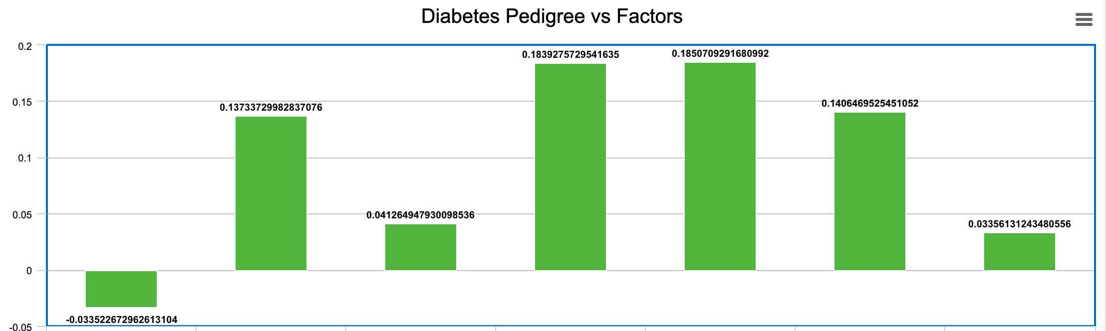
# What is the correlation between diabetes pedigree and other factors?
preg = datas['DiabetesPedigreeFunction'].corr(datas['Pregnancies'])
glucose = datas['DiabetesPedigreeFunction'].corr(datas['Glucose'])
bp = datas['DiabetesPedigreeFunction'].corr(datas['BloodPressure'])
st = datas['DiabetesPedigreeFunction'].corr(datas['SkinThickness'])
ins = datas['DiabetesPedigreeFunction'].corr(datas['Insulin'])
bmi = datas['DiabetesPedigreeFunction'].corr(datas['BMI'])
age = datas['DiabetesPedigreeFunction'].corr(datas['Age'])
print(preg, glucose, bp, st, ins, bmi, age)
# Which Age group has the highest average Glucose?
# Create AgeGroup column
datas = datas.copy()
datas['AgeGroup'] = pd.cut(
datas['Age'],
bins=[20, 30, 40, 50, 60, 100],
labels=['20s', '30s', '40s', '50s', '60+'],
right=False
)
glucose_by_age = datas.groupby('AgeGroup')['Glucose'].mean()
highest_glucose_group = glucose_by_age.idxmax()
print(highest_glucose_group)
# What percentage of people have BMI above 30 (obese)?
obese = datas[datas['BMI'] > 30]
obese_percentage = len(obese) / len(datas) * 100
print(obese_percentage)
master_function(datas)
-0.033522672962613104 0.13733729982837076 0.041264947930098536 0.1839275729541635 0.1850709291680992 0.1406469525451052 0.03356131243480556
50s
60.546875


/var/folders/93/y55vzx413xxdrd4m_6cv_rmm0000gn/T/ipykernel_13033/2651657759.py:26: FutureWarning: The default of observed=False is deprecated and will be changed to True in a future version of pandas. Pass observed=False to retain current behavior or observed=True to adopt the future default and silence this warning.
  glucose_by_age = datas.groupby('AgeGroup')['Glucose'].mean()
Chart:
SQL
import sqlite3
import pandas as pd
datas = pd.read_csv('/Users/maryamabdul-aziz/vscode/maryam_2025/_notebooks/data/diabetes.csv')

conn = sqlite3.connect(":memory:")

datas.to_sql("diabetes", conn, index=False, if_exists="replace")

query = "SELECT Outcome, AVG(Glucose) AS avg_glucose FROM diabetes GROUP BY Outcome"
result = pd.read_sql_query(query, conn)

print(result)
import sqlite3
import pandas as pd

data = pd.read_csv('/Users/maryamabdul-aziz/vscode/maryam_2025/_notebooks/data/diabetes.csv')

conn = sqlite3.connect(':memory:')

data.to_sql('diabetes', conn, index=False, if_exists='replace')

query = "SELECT * FROM diabetes WHERE Outcome = 1"
diabetic_patients = pd.read_sql_query(query, conn)
print(diabetic_patients)

query = """
SELECT AVG(Age) as AvgAge, AVG(BMI) as AvgBMI, COUNT(*) as Count
FROM diabetes
WHERE Outcome = 1
"""
diabetic_stats = pd.read_sql_query(query, conn)
print(diabetic_stats)

query = """
SELECT Outcome, COUNT(*) as Count
FROM diabetes
GROUP BY Outcome
"""
outcome_distribution = pd.read_sql_query(query, conn)

print(outcome_distribution)
     Pregnancies  Glucose  BloodPressure  SkinThickness  Insulin   BMI  \
0              6      148             72             35        0  33.6
1              8      183             64              0        0  23.3
2              0      137             40             35      168  43.1
3              3       78             50             32       88  31.0
4              2      197             70             45      543  30.5
..           ...      ...            ...            ...      ...   ...
263            1      128             88             39      110  36.5
264            0      123             72              0        0  36.3
265            6      190             92              0        0  35.5
266            9      170             74             31        0  44.0
267            1      126             60              0        0  30.1

     DiabetesPedigreeFunction  Age  Outcome
0                       0.627   50        1
1                       0.672   32        1
2                       2.288   33        1
3                       0.248   26        1
4                       0.158   53        1
..                        ...  ...      ...
263                     1.057   37        1
264                     0.258   52        1
265                     0.278   66        1
266                     0.403   43        1
267                     0.349   47        1

[268 rows x 9 columns]
      AvgAge     AvgBMI  Count
0  37.067164  35.142537    268
   Outcome  Count
0        0    500
1        1    268
- Discuss the advantages and disadvantages of using SQL versus Pandas for data analysis, focusing on performance, readability, and ease of use.
SQL is better for large datasets that need complicated queries and aggregations. It’s better for structure but can become difficult to use for advanced data manipulation. Pandas is better for smaller datasets because it’s flexible, allowing for quick analysis with Python. However, it can struggle with large data and become less efficient for complicated queries.